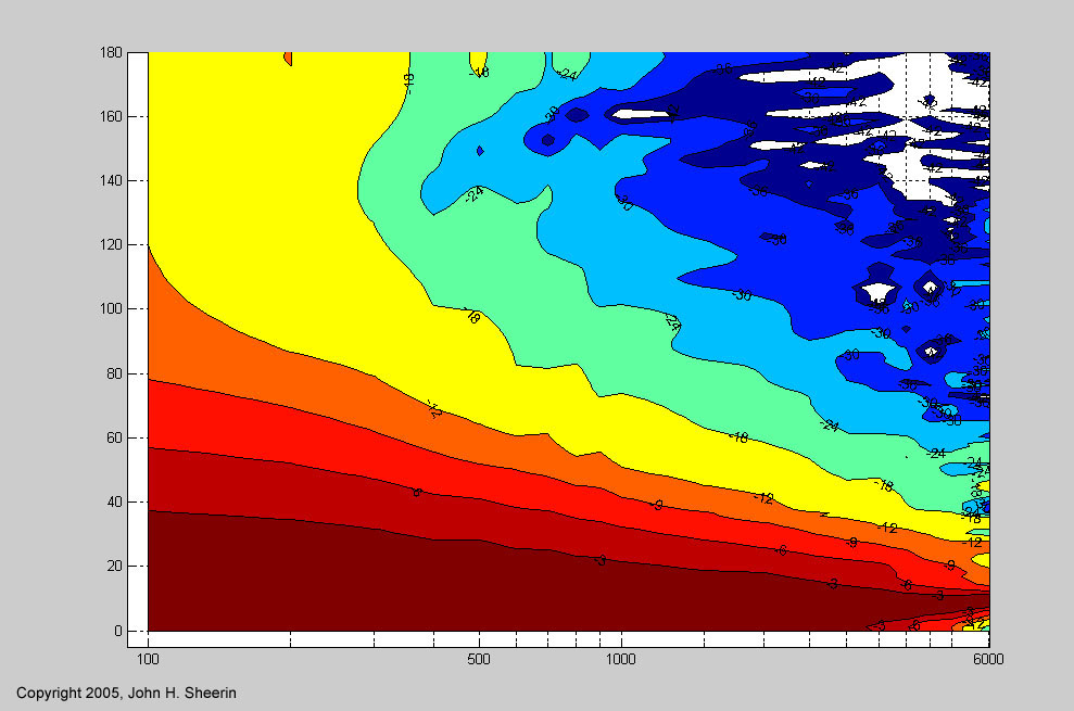
The plots linked below are polar maps of various horn and direct radiator geometries. A polar map is a way of showing the directional characteristics of a speaker. I first heard of it from Earl Geddes’ work. The x axis is frequency and the y axis is the angle from on-axis. The color or z data is the sound pressure level in decibels relative to 0dB. The contours are plotted through various sound pressure levels. -6dB is usually taken to be the angle of the radiation pattern, but this type of plot will show you a bit more information than that.

For the horns, the origin is taken to be the center of the mouth of the horn. For direct radiators, it is the center of the cone in the plane across the front of the driver’s frame. The SPL level has been normalized to be 0 dB at the point of maximum pressure at each frequency, but this is not necessarily on-axis. This has some implications in how you look at the data, but when you consider that you could equalize the on-axis response however you wanted, it is not such a big deal – you still are seeing the directional characteristics that exist. For example, on this Le Cleac'h horn the on-axis response falls off at high frequencies but there are lobes just off center that stay at the same 0dB level. In reality, you might choose to eq the on-axis response to be flat. However, there would still be lobes at those frequencies and angles, and they would be the greater in amplitude compared to the on-axis response by the amount shown in these graphs.

In cases where two horns / drivers are noted with a crossover frequency, the polar responses are actually just spliced together on the same graph - no crossover was simulated. That bit of programming is for another day. Some of the horns were also simulated with different wave shapes at the throat. This is what is meant by 'flat wave', etc. in the file names.

Polar maps